Processing Satellite Imagery for Deep Learning
For this project, I decided to model the relationship between NOAA Landsat imagery and building density in OpenStreetmap. I started by downloading large GeoTIF files from GloVis, a USGS tool for examining all kinds of remote sensing data. With the files in hand, I sorted through numerous band layers corresponding to different recorded wavelengths, and opted to use infrared band 10.
Reprojecting Coordinates
Images from this source used a different coordinate system, Universal Transverse Mercator (UTM), which describes locations as being a number of meters east and north of a southwest origin. For my purposes, which involved geographic data from another source, every location needed to be referenced in decimal degrees (13.581, 53.226). I used the Python library Rasterio to reproject GeoTIF images from one coordinate system to the other. Here, a function opens the source file, calculates the coordinate transformation between the two projections, and, and reprojects the image, saving it to a new folder.
for path in source_paths:
        print(f'reprojecting {path}')
        with rasterio.open(path) as src:
            transform, width, height = calculate_default_transform(src.crs, projection, src.width, src.height, *src.bounds)
            kwargs = src.meta.copy()
            kwargs.update({
                'crs': projection,
                'transform': transform,
                'width': width,
                'height': height
            })

            reproject_path = reproject_folder + '/' + clean_filename(path, keep_ext=True)
            print(f'reproject path: {reproject_path}')

            with rasterio.open(reproject_path, 'w', **kwargs) as dst:
                for i in range(1, src.count + 1):
                    reproject(
                        source=rasterio.band(src, i),
                        destination=rasterio.band(dst, i),
                        src_transform=src.transform,
                        src_crs=src.crs,
                        dst_transform=transform,
                        dst_crs=projection,
                        resampling=Resampling.nearest)
Storing Data Geographically
To facilitate the storage of data about each relevant area of the earth, I created a massive Numpy array. It contained 6480000 elements (1800*3600) and had a spot for info on every tenth-of-a-degree square in the decimal coordinate system. I filled the grid by iterating through every item, filling them with the coordinates of their southwest corner, a status variable for tracking processing progress, and several other items.
#create empty array
world = np.empty((rows, cols), dtype=object)
#copy start longitude to variable for iterator
lon = start_lon
#lat is adjusted down one tile so coordinates represent tile's southwest corner
lat = start_lat - increment
#iterate through entire array and write coordinates and default values
for row in range(world.shape[0]):
lat_entry = round(lat,1)
#calculate geographic area of one area in the array based on latitude
geo_area = latitude_to_area(lat_entry+increment/2, increment)
lat -= increment
for tile in range(world.shape[1]):
lon_entry = round(lon,1)
lon += increment
#write data to Numpy array
world[row][tile] = {'origin':(lon_entry, lat_entry), 'tile_path':'', 'image_path':'', 'status':0, 'geo_area':geo_area, 'buildings':-1}
#reset longitude at end of row
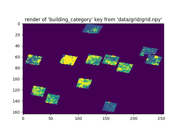
lon = start_lonHere is a Pyplot rendering of one variable in the grid, cropped for faster processing and analysis.
 </figure>
Each element of a Numpy array can only store one object, so I nested data inside a basic dictionary. The above render is of the values behind the dictionary key ‘building_category.’
Labeling
Once storage was allotted, I began by labeling each area with a one if it overlapped with available satellite imagery. This sped up later steps by eliminating the need for try/except blocks and attempting to load nonexistent images. I also added the filepath of the overlapping imagery for quick access later. Here is the statement that was run on each array element to determine its usefulness:
if grid[row][tile].get('status') == 0:
                    if grid[row][tile].get('origin')[0]>west and grid[row][tile].get('origin')[0]+increment<east:
                        if grid[row][tile].get('origin')[1]>south and grid[row][tile].get('origin')[1]+increment<north:
                            #flag area as containing image data
                            grid[row][tile]['status'] = 1
                            grid[row][tile]['image_path'] = image_path
Slicing into Tiles
To get bite-size imagery portions to model against OpenStreetMap, I built a function to crop out the image area overlapping each tile. It iterated through available reprojected images, generating a bounding box of four coordinates from the stored southwest coordinate and an increment variable (set to 1/10 of a degree). The bounding box was passed straight to Rasterio’s crop function, which created a new tile GeoTIF which was stored in a new folder. The status variable was also set to 2 to signify this development.
if grid[row][tile]['status'] == 1 and grid[row][tile]['image_path']==image_path:
                    tile_lon = grid[row][tile]['origin'][0]
                    tile_lat = grid[row][tile]['origin'][1]
                    bbox = corner_to_bbox((tile_lon,tile_lat), increment)
                    grid[row][tile]['tile_path'] = crop(image_path, tile_folder, bbox)
                    grid[row][tile]['status'] = 2
Check for Blank Tiles
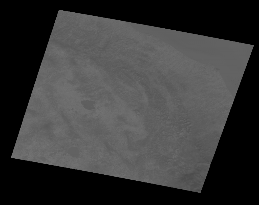
Now that the tiles were cropped, it was time to check if they contained useful information. Landsat satellites take imagery diagonally around the earth, and resulting images that are rotated to be the correct direction have large blank spots, like so:
 </figure>
To deal with this, I wrote a script to check if the number of blank, or zero pixels was below a certain threshold (5%). If valid, the corresponding areas would be be marked with status=3, representing the completion of this level of processing. Here is the code snippet that deals with that logic.
tile_array = rasterio.open(tile_path).read(1)
                blank_pixels = (tile_array == 0).sum()
                total_pixels = tile_array.shape[0] * tile_array.shape[1]
                blank_ratio = blank_pixels/total_pixels
                if blank_ratio < threshold:
                    grid[row][tile]['status'] = 3
Storing Data for Modeling
After performing a resizing operation on each tile to convert it from ~275 pixels square to 128 pixels square, I was ready to load image data into an array for modeling. Like many preceding functions, I iterated through the whole coordinate grid Numpy array, looking for areas with a status indicating full processing.
    #iterate through geographic grid and file data in lists
    grid = np.load(grid_path, allow_pickle=True)
    for row in range(grid.shape[0]):
        for tile in range(grid.shape[1]):
            if grid[row][tile].get('status') == 4:
                X.append(np.array(Image.open(grid[row][tile].get('prepared_path'))))
                y.append(grid[row][tile].get('building_category'))
From that point, I only had to:
- convert the resulting sample and label lists to Numpy arrays
- one-hot encode the labels
- add a required fourth dimension to the image sample array indicating a single frequency band
- min-max scale pixel values
The resulting data was now fit for modeling with any Keras neural net backend.
