Exploring Data Separability With Histograms
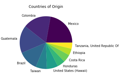
For my Flatiron School module 3 project, I decided to classify coffee samples from the Coffee Quality Institute by country. The dataset contained samples from numerous countries, but my analysis included only the top 1o most common producers in the set to make classification feasible. These countries were:
- Mexico
- Colombia
- Guatemala
- Brazil
- Taiwan
- United States (Hawaii)
- Honduras
- Costa Rica
- Ethiopia
- Tanzania
 </figure>
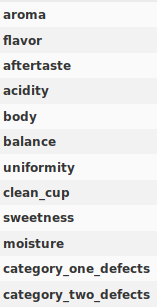
There were also >30 features for each sample, including growing altitude, preparation method, aroma, acidity, defects, etc. To manage complexity, I whittled that feature list down to attributes one could glean only by looking at or tasting the coffee. Things like flavor, acidity, moisture, defects. 12 features in all.
 </figure>
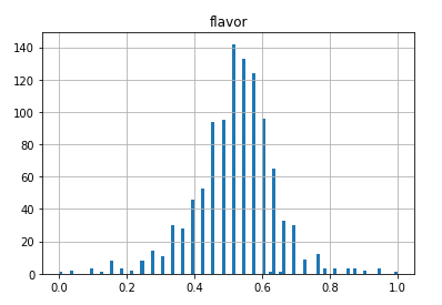
One of the first things I did with the data was to plot histograms of the data from each feature. Most of the information fell into normal distributions, but some turned out to be strongly exponential.
 </figure>
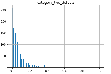
I also created a box plot for each feature and a multicollinearity matrix, but that’s all the exploration I did before moving on to modeling. This turned out to be a major mistake. If I had explored more deeply at this step, picking out the feature distributions by country and comparing them, I might have realized the futility of my country classification objective and revised the problem.
As I would find out later, the distribution means between countries for a given feature, like acidity, were extremely close. So close, that I doubt a human coffee expert could determine a coffee’s country of origin based on the numbers in this set.
After modeling the data with many different algorithms, like support vector classifiers, random forest classifiers, and gradient boosting classifiers, I became discouraged with the results. When I used proper cross-validation and hyperparameter optimization, accuracy scores never reached above 33%, only about 10% above the accuracy of picking Mexico as the origin of every sample!
At this point, I took a step back to design some new visualizations and came up with this.
 </figure>
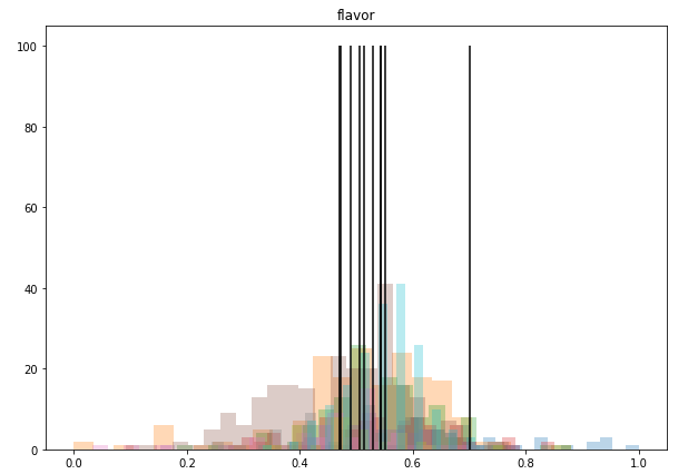
In this family of overlapped histograms, each country is represented by a color. I set the alpha of each distribution to o.03 so every bit of data can be seen through the crowd. The black vertical lines represent the means of each feature, which is what turned me on to the fact that coffee from different countries is nearly indistinguishable with this data alone.
Here is the code I used to iteratively create a meta-histogram from each feature in the dataset:
'''
Hists is a Pandas DataFrame made by recombining the target and features DataFrames. It represents all the data in this analysis.
'''

#iterate through every column in the features DataFrame
for feature in data_features.columns:
    #create pyplot figure and add axis
    fig = plt.figure(figsize=(10,7))
    ax = fig.add_subplot(111)
    #iterate through country labels
    for country in hists['country_of_origin'].unique():
        #get samples corresponding to particular country,
        #then single out a particular feature from those samples
        dist = hists.loc[hists['country_of_origin'] == country][feature]
        #plot a histogram with a low alpha for overlap visiblity
        ax.hist(dist, alpha=0.3, bins=25)
        #plot a vertical line representing the mean
        ax.vlines(dist.mean(), 0, 100)
    #set the title of the graph to the name of the feature
    ax.set_title(feature)
    #display the graph
    plt.show()
One problem I noticed when writing this post, was that there is no way to dynamically adjust the height of the vertical mean lines. Many of the graphs display nicely, but by hard-coding their height as 100, some histograms get squashed like the one above. A few graphs also tower above the lines, which is distracting and ugly.
 </figure>
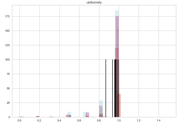
My initial fix was to replace the hard-coded height with the distribution mode, which was thoughtless, because the most common value has no relationship with how many of those common values there are.
After some research, I discovered a purpose built method called ‘axvline.’ It automates the tinkering I was doing with the ‘vlines’ method and simply draws a line from the top to the bottom of the axis.
ax.axvline(dist.mean(), c='black')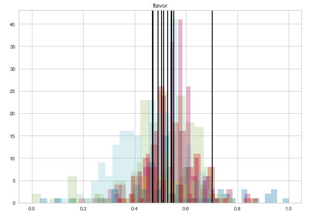
Now the country distribution mean lines go right to the top without stretching the graph.
Another objective I had was to determine what country that line out to the right represented. I set up a dictionary to record means by country, then print them out after each graph as a sort of legend.
"flavor" Means by Country:
------------------------------------------------
Ethiopia 0.7014876033057854
Guatemala 0.5140202020202014
Brazil 0.5430950728660647
United States (Hawaii) 0.5441594022415942
Costa Rica 0.5299108734402851
Mexico 0.47237288135593103
Honduras 0.4702797202797201
Taiwan 0.5048567870485677
Tanzania, United Republic Of 0.490818181818182
Colombia 0.5516741182314951
------------------------------------------------
It appears that Ethiopia outstrips the competition when it comes to flavor ratings! This was also true of a number of other features (aroma, aftertaste, acidity, body, and balance).
Here is the updated code:
#iterate through every column in the features DataFrame
for feature in data_features.columns:
    #create pyplot figure and add axis
    fig = plt.figure(figsize=(10,7))
    ax = fig.add_subplot(111)
    #iterate through country labels
    for country in hists['country_of_origin'].unique():
        #get samples corresponding to particular country,
        #then single out a particular feature from those samples
        dist = hists.loc[hists['country_of_origin'] == country][feature]
        #plot a histogram with a low alpha for overlap visiblity
        ax.hist(dist, alpha=0.3, bins=25)
        #plot a floor-to-ceiling vertical line
        ax.axvline(dist.mean(), c='black')
    #set the title of the graph to the name of the feature
    ax.set_title(feature)
    #display the graph
    plt.show()
    #print out a list of countries and their means for this feature
    print(f'"{feature}" Means by Country:')
    print('------------------------------------------------')
    for key, val in mean_dict.items():
        print(key, val)
    print('------------------------------------------------')
Check out my project on GitHub.
