Digging for business insights in the Northwind database
In this project, I was tasked with conducting four hypothesis tests on the Northwind SQL database. I used Python, Jupyter Notebooks, and SQL files to gather relevant data, process it into a usable form, and conduct various statistical tests. For each question, I will explain my methods, rationale, and findings.
Q1: Do discounts have a statistically significant effect on the number of products customers order? If so, at what level(s) of discount?
I did not write this question, but the idea behind it seems fairly obvious:
Is discounting products a viable way to increase sales?
For statistical analysis, though, the question has to be written more precisely than either of these renditions. In the first sentence of the original question, there are two important terms.
- Discounts
- Number of products customers order
We will define both of these quantities in terms of orders, as opposed to customers or line items within orders.
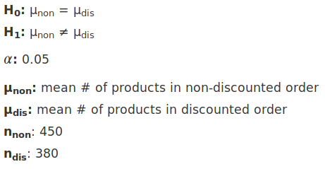
Discount will be defined as the total number of dollars off an order divided by the entire order value.
Number of products customers order will be defined as the number of products in a particular order.
Here are the parameters of the hypothesis test I set out to conduct:
 </figure>
For this analysis, I initially thought I would need four tables:
- Products
- Order Details
- Orders
- Customers
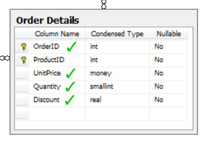
However, after examining the schema, I discovered that the Order Details table had everything I needed.
 </figure>
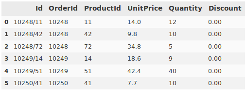
First, I imported the data into a Pandas DataFrame, then proceeded to create a new DataFrame as a container for the information after processing. Next, I wrote a script to iterate through the raw data, tabulate discounts and product quantities for each order, and write it to the results table. The data started out like this:
 </figure>
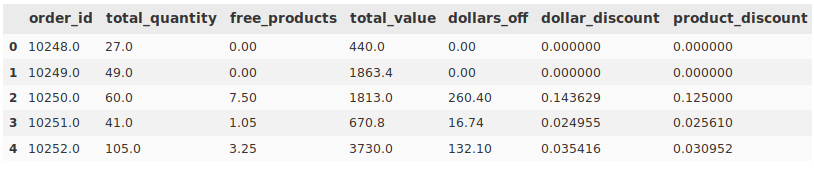
And after some processing, ended up like this:
 </figure>
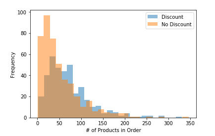
To answer the first part of the question, about whether having a discount has an effect, I split the data into discounted and non-discounted orders. Here is a histogram of that data:
 </figure>
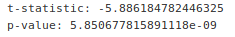
I used the scipy.stats.ttest_ind function to perform a two tailed t-test of these distributions, which yielded these results:
 </figure>
Since the p-value was much lower than our alpha, we could reasonably conclude that order discount has a statistically significant effect on the quantity of products in an order
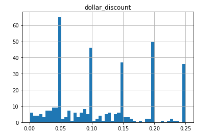
The second part of the question, which asked what levels of discount in particular have an effect, would involve a different kind of test. The first thing I did was to render a histogram of the distribution of discounts across all discounted orders.
 </figure>
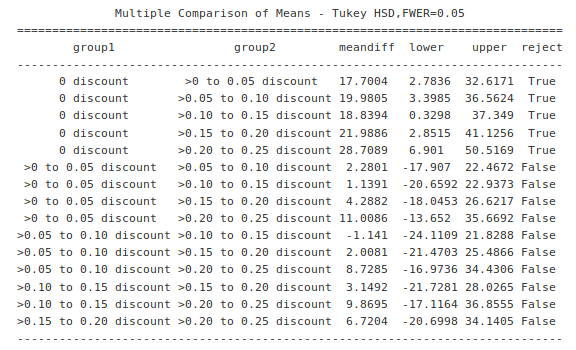
To compare differing levels of discount, I decided to use a Tukey test. For this test, I segmented orders with various levels of discount into bins 0f 0.05 width with statements like this:
q1_tukey_01to05 = q1_processed[(q1_processed['dollar_discount']>0) &
    (q1_processed['dollar_discount']<=0.05)]['total_quantity']
From there, I molded the data into the particular format that our Statsmodels function (statsmodels.stats.multicomp.pairwise_tukeyhsd) asked for, and ran the test. Here is the outcome.
 </figure>
All null hypotheses were rejected when orders with no discount were compared to orders with any level of discount. Based on this we can reasonably conclude that any level of discount has a statistically significant relationship with the number of products in an order.
Q2: Do orders contain a statistically significant different value of products when the employee responsible for the sale has the same phone area code as the customer?
The idea behind this question was that customers interacting with someone from their own region of the country or globe might have more amiable sales experiences, leading to more sales over time.
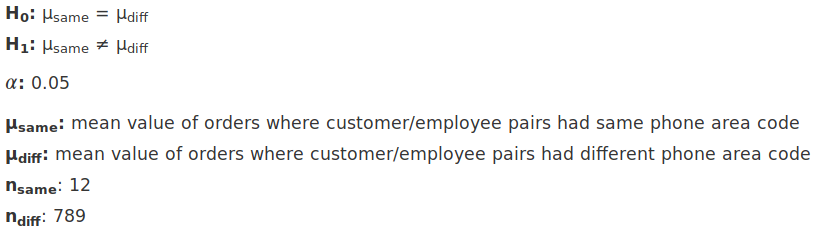
Here are the parameters of the hypothesis test I set out to conduct:
 </figure>
To get phone numbers of customers and employees, as well as customer order values, I had to join four tables:
- Order
- OrderDetail
- Customer
- Employee
As a challenge, I decided to do the bulk of my data wrangling in SQL rather than Pandas, which required two 19-line query files. Here is one of them:
--Calculate the value of each order line item, then sum all the values
--by order id as specified in the group by clause
SELECT SUM(OrderDetail.Quantity * OrderDetail.UnitPrice * (1-OrderDetail.Discount)) AS order_value
--Get data from orders table
FROM [Order]
--Join the other 3 tables on appropriate IDs
INNER JOIN OrderDetail ON [Order].Id=OrderDetail.OrderId
INNER JOIN Employee ON [Order].EmployeeId=Employee.Id
INNER JOIN Customer ON [Order].CustomerId=Customer.Id
--Request only records where phone area codes match
WHERE
    --Use SUBSTR to get area code from customer phone number
    SUBSTR(
        --Remove symbols from customer phone number for use as first arg in SUBSTR
        REPLACE(REPLACE(REPLACE(REPLACE(
        Customer.Phone,'-',' '),')',''),'(',''),'.',' '),
        --Start slice at string index 1
        1,
        --Find slice end index using INSTR
        INSTR(
            --Remove symbols from customer phone number again to provide
            --phone # string identical to the one cleaned above
            REPLACE(REPLACE(REPLACE(REPLACE(
            Customer.Phone,'-',' '),')',''),'(',''),'.',' '),
            --Ask INSTR to search for the space after the area code and provide its index
            " "
        )
    )
    --Compare customer and employee area codes
    =
    --Use SUBSTR to get area code from employee phone number
    SUBSTR(
        --Remove symbols from employee phone number for use as first arg in SUBSTR
        REPLACE(REPLACE(REPLACE(REPLACE(
        Employee.HomePhone,'-',' '),')',''),'(',''),'.',' '),
        --Start slice at string index 1
        1,
        --Find slice end index using INSTR
        INSTR(
            --Remove symbols from employee phone number again to provide
            --phone # string identical to the one cleaned above
            REPLACE(REPLACE(REPLACE(REPLACE(
            Employee.HomePhone,'-',' '),')',''),'(',''),'.',' '),
            --Ask INSTR to search for the space after the area code and provide its index
            " "
        )
    )
--Group all data by its order id, working in concert with SELECT,
--which sums up the value of each order
GROUP BY [Order].Id
Most of the lines in the query fall within the WHERE clause. Here, each phone number is taken through four layers of REPLACE functions to remove various symbols (many of the numbers were formatted differently). After that, INSTR and SUBSTR were used to locate the end of the area code and extract it from the rest of the phone number. Next, the area codes of customers and employees were compared. I wrote the above query file to fetch records with matching area codes, and another almost identical file to fetch those without a match.
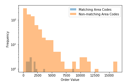
Initially, I compared these two distributions with a histogram:
 </figure>
I had to use a log scale on the y axis because there were so many more non-matching records than matching records.
Because the samples were so varied in size (n=12 versus n=789) I decided to use the non-parametric Mann-Whitney U Test (scipy.stats.mannwhitneyu). This was the result:
P = 0.08210731477282339
Because P was greater than our alpha of 0.05, we cannot reject the null hypothesis. This means that whether a customer and employee share a phone area code does not have a statistically significant effect on the value of products ordered. However, this result should be taken with a grain of salt, as one of the distributions had only 12 data points.
Q3: Do products in the greater half by quantity sold have a statistically significant different reorder threshold than those in the lesser half by quantity sold?
The intent behind this question was to find out whether products that are more popular have reorder thresholds that reflect their popularity. If a product is more popular, consistently having it in stock would require a higher threshold, and would result in more satisfied customers.
I used 3 tables in this analysis:
- Product
- OrderDetail
- Order
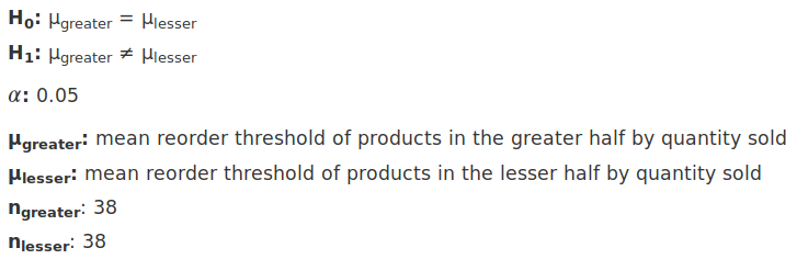
Here are the parameters of the hypothesis test I set out to conduct:
 </figure>
Here is the SQL I used to retrieve data for the upper half of orders by value:
SELECT Product.ReorderLevel
    FROM Product
    JOIN OrderDetail ON Product.Id=OrderDetail.ProductId
    JOIN [Order] ON [Order].Id=OrderDetail.OrderId
GROUP BY Product.Id
ORDER BY SUM(OrderDetail.Quantity) ASC
LIMIT 38
LIMIT 38 was used instead of a dynamic limit like TOP 50 PERCENT because SQLite does not have such a feature.
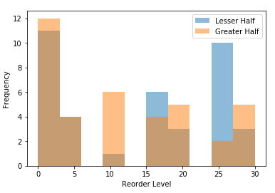
After getting the data from the bottom half of orders by value, I rendered the distributions in histograms.
 <figcaption>overlapping</figcaption></figure>
 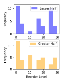 <figcaption>separate</figcaption>
I used the scipy.stats.ttest_ind function again to calculate whether the difference between these two distributions was statistically significant. Because they were so similar, it returned a value of:
P = 0.40382632307192035
This was significantly higher than the alpha of 0.05, so the null hypothesis stands. Whether a product is in the greater or lesser half of products by quantity sold does not have a statistically significant relationship with the reorder threshold
Q4: Do customers with streaks of selecting the same shipper 5 or more times in a row have a statistically significant difference in lifetime sales value (loyalty)?
I wondered if I could find a proxy for loyalty or lifetime sales value for a customer outside of the actual sales history. I decided to use whether a customer chooses the same shipping option 5x in a row as a potential predictor. Inherent in this question is the assumption that the customer is the one choosing shipping options, which may not be true, but I thought it worth some exploration.
I used 3 tables in this analysis:
- Order
- OrderDetail
- Customer
Here are the parameters of the hypothesis test I set out to conduct:
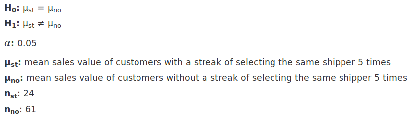 </figure>
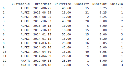
I used SQL to join all 3 tables, ordering by customer id and order date to make processing easier.
SELECT CustomerId, OrderDate, UnitPrice, Quantity, Discount, ShipVia
      FROM [Order]
INNER JOIN Customer ON [Order].CustomerId = Customer.Id
INNER JOIN OrderDetail on [Order].Id = OrderDetail.OrderId
  ORDER BY CustomerId, OrderDate
Here is some output from that statement:
 </figure>
The rest of the processing was done in Pandas, where I iterated through the data to tally customer value and shipping streaks. This information was saved to a results DataFrame with one row per customer.
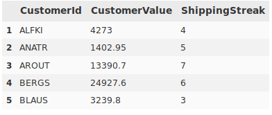 </figure>
After some double-checking to ensure the accuracy of the data after processing, I moved on to visualization.
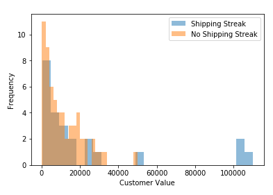 </figure>
Lastly, I used a t-test to test our hypothesis, which resulted in:
P = 0.09273245000580074
The P value exceeded our alpha of 0.05, so whether a customer has a streak of selecting the same shipper 5 times in a row does not have a statistically significant relationship with that customer’s lifetime dollar value.
In conclusion, none of my own hypothesis tests yielded statistically significant results, but that is okay. With more time, I would like to tweak a few questions and set different thresholds. For example:
- Using area code geocoding to plot coordinates for employees and customers, then setting a distance threshold
- Comparing the top and bottom quarters of orders to check for differences in reorder threshold
- Redefining a shipping streak as 3 or 7 selections of the same shipper, instead of 5
Happy programming!
