Converting dates to floating point numbers with Python’s datetime library
The Method
While cleaning the data for my recent house price prediction project, I came across an issue involving different date formats. There were two relevant time-related columns in the data: ‘date’, which represented the date each house was sold, and ‘yr_built’, which represented the year each house was constructed. ‘ The ‘yr_built’ values were stored as integers, ready to be visualized and modeled, but every ‘year’ value was stuck in classic mm/dd/yyyy format.
To parse these date strings, I imported Python’s ‘datetime‘ library.
import datetime as dtPerusing the ‘datetime’ documentation, the strptime() method immediately stood out to me
 </figure>
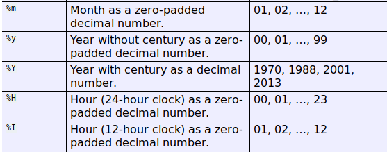
It accepts the string to be manipulated as the first argument, and a specialized format string as the second. Section 8.1.7 provides an entire table of codes for parsing dates with these functions. These codes have a similar format to “% substitutions” that have long been used for formatting strings in Python.
 </figure>
Starting with a value like 01/23/2019, here is how the datetime.strptime() method would be used to parse out the constituent parts of the date.
dt_obj = dt.datetime.strptime(date_string, '%m/%d/%Y')“%m” tells the method to extract a two digit month, while “%d” tells it to extract a two digit day and “%Y” a four digit year. All this time information is then stored as a datetime object in variable “dt_obj.”
type(dt_obj)

datetime.datetime
There are a number of useful functions for outputting date information in different forms. For example, “datetime.isoformat()” produces an ISO 8601 yyyy-mm-dd formatted date string. The format we want though, is somewhat peculiar, and not covered completely by a single “datetime” function. Conveniently, datetime objects have ‘year’,’month’, and ‘day’ attributes. By processing these attributes into decimals of a year, and adding them together, we arrive at the floating point year value we are seeking.
return dt_obj.year + (dt_obj.month-1)/12 + (dt_obj.day-1)/365.25The way people speak and write about years, months, and days, is a little different from the way they are recorded in computers. When we say that it is January 19th, 2014, we mean that we are inside of the 2014th year A.D. Recording a date in float format (essentially # of years A.D.) requires us to record this date as two thousand and thirteen years plus whatever portion of the year 2014 has occurred. This threw me through a loop when I first encountered my function’s output, because I was not expecting a year output of 2013 for a date in 2014. The expression above adds together values for year, month, and day, which are calculated by dividing the time unit by how many of them there are in a year (years/1, months/12, days/365.25). Before division, one is subtracted from months and from days. This is because, until a time unit is completed, it cannot be counted. Years should also have had one subtracted, but in my initial code, the year output confused me. Here’s an updated version:
return dt_obj.year-1 + (dt_obj.month-1)/12 + (dt_obj.day-1)/365.25As a side note, days is divided by 365.25 to account for leap years.
The Purpose
This whole date conversion process was to convert one feature of my dataset (year sold) into a format that could interact with another feature (year built). After the conversion, the former contained floats and the latter contained integers. I figured that I could engineer a useful feature, ‘age’, by subtracting the build date of each house from the sale date.
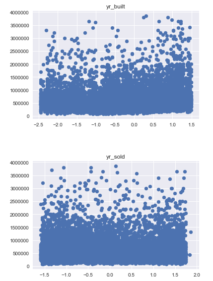
scaled_log_data['age'] = data.yr_sold - data.yr_builtHere is the scatter plots of ‘yr_built’ and ‘yr_sold’ versus our target variable ‘price’.
 </figure>
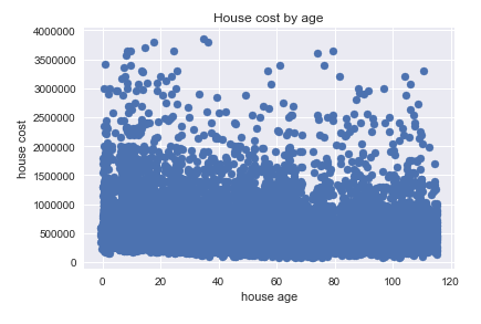
And here is the scatter plot of our newly engineered variable, ‘age’, versus the target ‘price’.
 </figure>
Unfortunately, our engineered variable does not yield a noticeably better relationship with price than the variables we started with. I imagine this is largely because of the small range of sale dates in the set. Every sale date in the set fell between the years 2014 and 2015. A variation this small relative to the decades-wide range of build dates in the set makes ‘yr_sold’, for all practical purposes, into a constant. The age graph would look very similar if we had simply subtracted every ‘yr_built’ value from the number 2014.
The Musings
Imagine, however, that we had a dataset with all the home sales of the last century in King County, Washington. How would sale price change as houses age? Would the home buyers of different decades have a penchant for houses of differing ages? How does the scatter of prices change as houses get older?
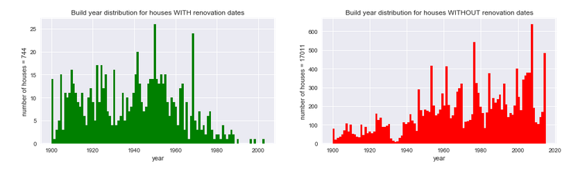
Another date variable in the dataset was ‘yr_renovated’. I opted not to include this feature in my analysis because only 3.44% of houses had renovation dates, but some early visualizations illustrated the utility of such information.
 </figure>
In these histograms, I presented a distribution of build dates for houses with and without renovations. The right chart seems to follow expectations: the further back in time we go, the fewer extant homes there are. If you don’t renovate your old house, it’s less likely to weather the years. On the left, however, we find an interesting distribution. It’s obvious that newer houses are much less likely to have been renovated, but as we go into the past, the renovation rates of different decades varies widely. For example, homes built in the late 40’s and early 50’s were more popular to renovate than those of any other decade in the set.
I hope this article has been informative for you and given you a few ideas for processing date features in your own dataset. Focusing in on just a few variables in this project has grown my appreciation for the creative potential of the data science profession, and I can’t wait to start my next analysis in a month or so!
